Tutorial#
Introduction#
This notebook will provide a step-by-step tutorial for using the caterpillard package to create the Caterpillar Diagram as proposed in the research article.
A Caterpillar Diagram is a visualization technique used for analyzing univariate time-series data. It consists of a series of colored circles with varying radii. The circle’s color represents the direction of change in the time-series data, and the circle’s size shows its variation.
It implements the innovative and intuitive Difference of Differences (DoD) approach to create a color schema. As proposed, it segregates the time-series data under analysis into a cohort of three consecutive time units. Further, it utilizes the unsigned differences between observations to assign a size to each cohort. This novel visualization technique can segregate the time-series data using seven colors or five stages of Aggressive, Ascent, Descent, Controlled, and Status Quo.
Further, the proposed mechanism utilizes the accumulated color information regarding each cohort to forecast the next step transition using a stationary matrix of Markov Chains.
[1]:
import numpy as np
import pandas as pd

from caterpillard import CaterpillarDiagram
Relative Analysis#
The Caterpillar Diagram can analyze a collection of time-series dataset together and produce a visualization for the user-defined data series out of them. This kind of analysis is termed here as relative analysis.
An example dataset is provided with the package which can be imported using from caterpillard import load_dataframe
[2]:
from caterpillard import load_dataframe
DataFrame info#
As shown in the output of info command above, the dataframe is a wide form dataset where each column stores the repeated response of each item (row) over the years. The package requires the dataframe in this format to create the diagram. This dataframe has 205 distinct entities in the index which will serve as an identification information for selecting the collection of time-series to work with. There are 49 columns in the dataset each reporting a numeric observation.
[3]:
df = load_dataframe()
print(df.info())
<class 'pandas.core.frame.DataFrame'>
Int64Index: 205 entries, 4 to 499
Data columns (total 49 columns):
 #   Column  Non-Null Count  Dtype
---  ------  --------------  -----
 0   1970    205 non-null    int64
 1   1971    205 non-null    int64
 2   1972    205 non-null    int64
 3   1973    205 non-null    int64
 4   1974    205 non-null    int64
 5   1975    205 non-null    int64
 6   1976    205 non-null    int64
 7   1977    205 non-null    int64
 8   1978    205 non-null    int64
 9   1979    205 non-null    int64
 10  1980    205 non-null    int64
 11  1981    205 non-null    int64
 12  1982    205 non-null    int64
 13  1983    205 non-null    int64
 14  1984    205 non-null    int64
 15  1985    205 non-null    int64
 16  1986    205 non-null    int64
 17  1987    205 non-null    int64
 18  1988    205 non-null    int64
 19  1989    205 non-null    int64
 20  1990    205 non-null    int64
 21  1991    205 non-null    int64
 22  1992    205 non-null    int64
 23  1994    205 non-null    int64
 24  1995    205 non-null    int64
 25  1996    205 non-null    int64
 26  1997    205 non-null    int64
 27  1998    205 non-null    int64
 28  1999    205 non-null    int64
 29  2000    205 non-null    int64
 30  2001    205 non-null    int64
 31  2002    205 non-null    int64
 32  2003    205 non-null    int64
 33  2004    205 non-null    int64
 34  2005    205 non-null    int64
 35  2006    205 non-null    int64
 36  2007    205 non-null    int64
 37  2008    205 non-null    int64
 38  2009    205 non-null    int64
 39  2010    205 non-null    int64
 40  2011    205 non-null    int64
 41  2012    205 non-null    int64
 42  2013    205 non-null    int64
 43  2014    205 non-null    int64
 44  2015    205 non-null    int64
 45  2016    205 non-null    int64
 46  2017    205 non-null    int64
 47  2018    205 non-null    int64
 48  2019    205 non-null    int64
dtypes: int64(49)
memory usage: 80.1 KB
None
Initialization#
The generation of the Caterpillar diagram requires a series of steps. The first step is to initialize the CaterpillarDiagram class with the required parameters, data, relative, and the optional output_path.
Select the sub-collection of data series from the data frame as the input for the data parameter and assign True to the relative parameter because we are performing the relative analysis.
Here, we select indexes (4, 19, 25, 92, 122, 129, 141, 153, 186) from the data frame for relative analysis.
[4]:
df_subset = df[df.index.isin([4, 19, 25, 92, 122, 129, 141, 153, 186])]
print(df_subset.info())
<class 'pandas.core.frame.DataFrame'>
Int64Index: 9 entries, 4 to 186
Data columns (total 49 columns):
 #   Column  Non-Null Count  Dtype
---  ------  --------------  -----
 0   1970    9 non-null      int64
 1   1971    9 non-null      int64
 2   1972    9 non-null      int64
 3   1973    9 non-null      int64
 4   1974    9 non-null      int64
 5   1975    9 non-null      int64
 6   1976    9 non-null      int64
 7   1977    9 non-null      int64
 8   1978    9 non-null      int64
 9   1979    9 non-null      int64
 10  1980    9 non-null      int64
 11  1981    9 non-null      int64
 12  1982    9 non-null      int64
 13  1983    9 non-null      int64
 14  1984    9 non-null      int64
 15  1985    9 non-null      int64
 16  1986    9 non-null      int64
 17  1987    9 non-null      int64
 18  1988    9 non-null      int64
 19  1989    9 non-null      int64
 20  1990    9 non-null      int64
 21  1991    9 non-null      int64
 22  1992    9 non-null      int64
 23  1994    9 non-null      int64
 24  1995    9 non-null      int64
 25  1996    9 non-null      int64
 26  1997    9 non-null      int64
 27  1998    9 non-null      int64
 28  1999    9 non-null      int64
 29  2000    9 non-null      int64
 30  2001    9 non-null      int64
 31  2002    9 non-null      int64
 32  2003    9 non-null      int64
 33  2004    9 non-null      int64
 34  2005    9 non-null      int64
 35  2006    9 non-null      int64
 36  2007    9 non-null      int64
 37  2008    9 non-null      int64
 38  2009    9 non-null      int64
 39  2010    9 non-null      int64
 40  2011    9 non-null      int64
 41  2012    9 non-null      int64
 42  2013    9 non-null      int64
 43  2014    9 non-null      int64
 44  2015    9 non-null      int64
 45  2016    9 non-null      int64
 46  2017    9 non-null      int64
 47  2018    9 non-null      int64
 48  2019    9 non-null      int64
dtypes: int64(49)
memory usage: 3.5 KB
None
[5]:
cd = CaterpillarDiagram(data=df_subset, relative=True, output_path="/tmp/tut_output/")
Data Summary#
Use the data_summary method available in the class object to get info regarding the input data for analysis
[6]:
cd.data_summary()
Summarizing Data
<class 'pandas.core.frame.DataFrame'>
Int64Index: 9 entries, 4 to 186
Data columns (total 49 columns):
 #   Column  Non-Null Count  Dtype
---  ------  --------------  -----
 0   1970    9 non-null      int64
 1   1971    9 non-null      int64
 2   1972    9 non-null      int64
 3   1973    9 non-null      int64
 4   1974    9 non-null      int64
 5   1975    9 non-null      int64
 6   1976    9 non-null      int64
 7   1977    9 non-null      int64
 8   1978    9 non-null      int64
 9   1979    9 non-null      int64
 10  1980    9 non-null      int64
 11  1981    9 non-null      int64
 12  1982    9 non-null      int64
 13  1983    9 non-null      int64
 14  1984    9 non-null      int64
 15  1985    9 non-null      int64
 16  1986    9 non-null      int64
 17  1987    9 non-null      int64
 18  1988    9 non-null      int64
 19  1989    9 non-null      int64
 20  1990    9 non-null      int64
 21  1991    9 non-null      int64
 22  1992    9 non-null      int64
 23  1994    9 non-null      int64
 24  1995    9 non-null      int64
 25  1996    9 non-null      int64
 26  1997    9 non-null      int64
 27  1998    9 non-null      int64
 28  1999    9 non-null      int64
 29  2000    9 non-null      int64
 30  2001    9 non-null      int64
 31  2002    9 non-null      int64
 32  2003    9 non-null      int64
 33  2004    9 non-null      int64
 34  2005    9 non-null      int64
 35  2006    9 non-null      int64
 36  2007    9 non-null      int64
 37  2008    9 non-null      int64
 38  2009    9 non-null      int64
 39  2010    9 non-null      int64
 40  2011    9 non-null      int64
 41  2012    9 non-null      int64
 42  2013    9 non-null      int64
 43  2014    9 non-null      int64
 44  2015    9 non-null      int64
 45  2016    9 non-null      int64
 46  2017    9 non-null      int64
 47  2018    9 non-null      int64
 48  2019    9 non-null      int64
dtypes: int64(49)
memory usage: 3.5 KB
Generate Color Schema#
[7]:
cd.color_schema()
<class 'pandas.core.frame.DataFrame'>
Int64Index: 423 entries, 0 to 46
Data columns (total 8 columns):
 #   Column      Non-Null Count  Dtype
---  ------      --------------  -----
 0   d11         423 non-null    int64
 1   d12         423 non-null    int64
 2   d2          423 non-null    int64
 3   data_index  423 non-null    int64
 4   Cohort      423 non-null    object
 5   color       423 non-null    object
 6   level       423 non-null    object
 7   n_color     423 non-null    int64
dtypes: int64(5), object(3)
memory usage: 29.7+ KB
The color_schema method has implemented the DoD approach and created a data frame complete_cohort_df available as the instance attribute to the class object cd as shown below.
The column \(d_{11}\), \(d_{12}\) are the first differences and \(d_2\) is the second difference, respectively. The data_index column shows the index of the subset of the data frame that we selected earlier.
The Cohort column marks the cohort number for which the row of this data frame (complet_cohort_df) is storing the information. The columns color, level, and n_color stores the color and level information for the particular cohort as assigned by the DoD approach.
[8]:
cd.complete_cohort_df.head()
[8]:
| d11 | d12 | d2 | data_index | Cohort | color | level | n_color | |
|---|---|---|---|---|---|---|---|---|
| 0 | 0 | 0 | 0 | 4 | Cohort1 | grey | level7 | 7 |
| 1 | 0 | 2 | 2 | 4 | Cohort2 | red | level1 | 1 |
| 2 | 2 | -2 | -4 | 4 | Cohort3 | cyan | level4 | 4 |
| 3 | -2 | 0 | 2 | 4 | Cohort4 | blue | level5 | 5 |
| 4 | 0 | 0 | 0 | 4 | Cohort5 | grey | level7 | 7 |
Caterpillar Size#
The class object has a method named caterpillar_size which facilitates the size assignment to each cohort. Only four radii lengths can be assigned to a cohort based on the dispersion in the unsigned differences of consecutive observations in the time series. Please refer to the original article or source code for implementation details.
[9]:
cd.caterpillar_size()
Calculating sizes for each cohort
The above method will update the instance attribute complete_cohort_df with size information for each cohort.
[10]:
cd.complete_cohort_df.head()
[10]:
| d11 | d12 | d2 | data_index | Cohort | color | level | n_color | d11_radius | d12_radius | final_cohort_radius | |
|---|---|---|---|---|---|---|---|---|---|---|---|
| 0 | 0 | 0 | 0 | 4 | Cohort1 | grey | level7 | 7 | 4 | 4 | 4.0 |
| 1 | 0 | 2 | 2 | 4 | Cohort2 | red | level1 | 1 | 4 | 4 | 4.0 |
| 2 | 2 | -2 | -4 | 4 | Cohort3 | cyan | level4 | 4 | 4 | 4 | 4.0 |
| 3 | -2 | 0 | 2 | 4 | Cohort4 | blue | level5 | 5 | 4 | 4 | 4.0 |
| 4 | 0 | 0 | 0 | 4 | Cohort5 | grey | level7 | 7 | 4 | 4 | 4.0 |
Since each cohort contains two first differences, \(d_{11}\) and \(d_{12}\), the package will assign the radius to each of them. The final radius of the cohort is the mean of these two radii stored in final_cohort_radius.
Caterpillar Diagram Generation#
The class object provides the generate method to create and store the caterpillar diagram of the user-defined entity from the collection of time-series data which was provided as input.
[11]:
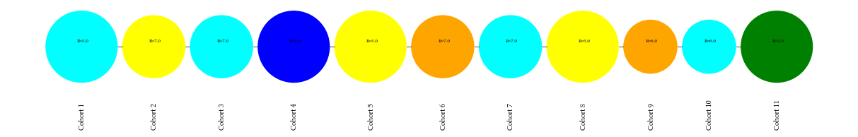
# Caterpillar diagram for entity 92 based on relative analysis
# Showing last 11 cohorts out of available 47 cohorts
cd.generate(data_index=92, n_last_cohorts=11)
[12]:
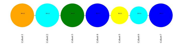
# Caterpillar diagram for entity 153 based on relative analysis
# Showing last seven cohorts out of available 47 cohorts
cd.generate(data_index=153, n_last_cohorts=7)
Color Schema Transitions#
The schema_transitions method will count the occurrence of transition from a particular color in a cohort to another color in the next consecutive cohort and creates a transition matrix for applying Markov Chains.
The relative analysis will utilize the color transitions of all the entities under analysis to forecast the next state transition.
[13]:
cd.schema_transitions()
Finding transitions
[14]:
# Instance attribute transition_mat stores the matrix
cd.transition_mat
[14]:
| red | orange | yellow | cyan | blue | green | grey | |
|---|---|---|---|---|---|---|---|
| red | 13 | 13 | 0 | 36 | 0 | 0 | 0 |
| orange | 10 | 1 | 0 | 16 | 0 | 0 | 0 |
| yellow | 21 | 13 | 0 | 25 | 1 | 0 | 1 |
| cyan | 0 | 0 | 40 | 0 | 28 | 8 | 1 |
| blue | 3 | 0 | 16 | 0 | 5 | 3 | 11 |
| green | 0 | 0 | 6 | 0 | 4 | 1 | 1 |
| grey | 15 | 0 | 0 | 0 | 0 | 0 | 130 |
For example, the matrix above shows that red has transitioned 36 times to the cyan color.
The above matrix facilitates creating the stationary matrix for the Markov chain.
Stationary Matrix#
[15]:
# n_sim_iter is the number of times the transition_mat
# will be multiplied by itself to reach a stationary state

cd.stationary_matrix(n_sim_iter=10**4)
Finding stationary matrix
100% (10000 of 10000) |##################| Elapsed Time: 0:00:12 Time: 0:00:12
[15]:
| red | orange | yellow | cyan | blue | green | grey | |
|---|---|---|---|---|---|---|---|
| red | 0.148306 | 0.065532 | 0.150192 | 0.186501 | 0.092087 | 0.029069 | 0.328313 |
| orange | 0.148306 | 0.065532 | 0.150192 | 0.186501 | 0.092087 | 0.029069 | 0.328313 |
| yellow | 0.148306 | 0.065532 | 0.150192 | 0.186501 | 0.092087 | 0.029069 | 0.328313 |
| cyan | 0.148306 | 0.065532 | 0.150192 | 0.186501 | 0.092087 | 0.029069 | 0.328313 |
| blue | 0.148306 | 0.065532 | 0.150192 | 0.186501 | 0.092087 | 0.029069 | 0.328313 |
| green | 0.148306 | 0.065532 | 0.150192 | 0.186501 | 0.092087 | 0.029069 | 0.328313 |
| grey | 0.148306 | 0.065532 | 0.150192 | 0.186501 | 0.092087 | 0.029069 | 0.328313 |
The above matrix is the final stationary matrix for all the entities taken together as input for the current relative analysis.
Absolute Analysis#
The Caterpillar Diagram can analyze a single data series and produce a visualization. This kind of analysis is termed here as absolute analysis. The transition matrix of the single time series data will facilitate the forecast of the next-step transition based on this single data series only.
The caterpillard package provides the single data series as an example dataset with the load_series function.
[16]:
from caterpillard import load_series
[17]:
data_ser = load_series()
[18]:
print(data_ser)
1970       0
1971       0
1972       1
1973       0
1974       0
1975      13
1976       1
1977       1
1978       0
1979     134
1980      74
1981     100
1982     307
1983     445
1984    1110
1985     279
1986    1279
1987    2137
1988    4307
1989    3743
1990    4136
1991    5026
1992    4622
1994    1687
1995    1878
1996    2872
1997    4168
1998    1702
1999    2198
2000    3020
2001    3478
2002    3231
2003    2909
2004    2119
2005    2837
2006    4533
2007    3274
2008    4919
2009    4190
2010    4259
2011    3296
2012    2408
2013    3208
2014    3524
2015    3090
2016    3673
2017    3681
2018    3152
2019    2336
Name: 92, dtype: int64
[30]:
data_ser.index
[30]:
Index(['1970', '1971', '1972', '1973', '1974', '1975', '1976', '1977', '1978',
       '1979', '1980', '1981', '1982', '1983', '1984', '1985', '1986', '1987',
       '1988', '1989', '1990', '1991', '1992', '1994', '1995', '1996', '1997',
       '1998', '1999', '2000', '2001', '2002', '2003', '2004', '2005', '2006',
       '2007', '2008', '2009', '2010', '2011', '2012', '2013', '2014', '2015',
       '2016', '2017', '2018', '2019'],
      dtype='object')
Initialization#
Similar to the approach discussed for relative analysis, the CaterpillarDiagram class accepts three arguments, viz. data for providing Pandas Series. The parameter relative should be False to mark this as an Absolute analysis. The parameter output_path is optional. When undefined by the user, the package will create an output directory, caterpillard_output.
[19]:
cd_absolute = CaterpillarDiagram(data=data_ser, relative=False, output_path="/tmp/tut_output/")
Data Summary#
[20]:
cd_absolute.data_summary()
Summarizing Data
Generate Color Schema#
The color_schema method will evaluate the color for each cohort.
[22]:
cd_absolute.color_schema()
The complete_cohort_df has first and second differences for the input data series with the assigned color, level, and n_color for each cohort.
[23]:
cd_absolute.complete_cohort_df.head()
[23]:
| d11 | d12 | d2 | Cohort | color | level | n_color | |
|---|---|---|---|---|---|---|---|
| 0 | 0.0 | 1.0 | 1.0 | Cohort1 | red | level1 | 1 |
| 1 | 1.0 | -1.0 | -2.0 | Cohort2 | cyan | level4 | 4 |
| 2 | -1.0 | 0.0 | 1.0 | Cohort3 | blue | level5 | 5 |
| 3 | 0.0 | 13.0 | 13.0 | Cohort4 | red | level1 | 1 |
| 4 | 13.0 | -12.0 | -25.0 | Cohort5 | cyan | level4 | 4 |
Caterpillar Size#
[24]:
cd_absolute.caterpillar_size()
Calculating sizes for each cohort
The caterpillar_size method will update the complete_cohort_df instance attribute.
[25]:
cd_absolute.complete_cohort_df.head()
[25]:
| d11 | d12 | d2 | Cohort | color | level | n_color | d11_radius | d12_radius | final_cohort_radius | |
|---|---|---|---|---|---|---|---|---|---|---|
| 0 | 0.0 | 1.0 | 1.0 | Cohort1 | red | level1 | 1 | 2 | 2 | 2.0 |
| 1 | 1.0 | -1.0 | -2.0 | Cohort2 | cyan | level4 | 4 | 2 | 2 | 2.0 |
| 2 | -1.0 | 0.0 | 1.0 | Cohort3 | blue | level5 | 5 | 2 | 2 | 2.0 |
| 3 | 0.0 | 13.0 | 13.0 | Cohort4 | red | level1 | 1 | 2 | 2 | 2.0 |
| 4 | 13.0 | -12.0 | -25.0 | Cohort5 | cyan | level4 | 4 | 2 | 2 | 2.0 |
Caterpillar Diagram Generation#
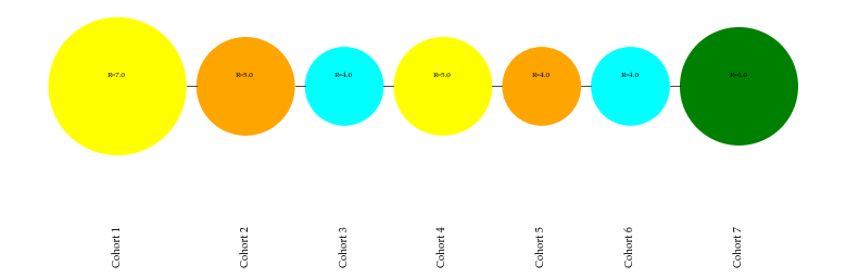
In the Absolute analysis, the generate method should not provide the data_index as it is a single data series. Further, if the data series is very long, then the user can provide the integer n_last_cohort to generate only the specified number of the cohort from the end.
[26]:
cd_absolute.generate(data_index=None, n_last_cohorts=7)
Color Schema Transitions#
The schema_transitions method will count the color change in the consecutive cohorts and create a matrix, as shown below. The generated matrix is available for the user by transition_mat as the instance attribute.
[27]:
cd_absolute.schema_transitions()
Finding transitions
[28]:
cd_absolute.transition_mat
[28]:
| red | orange | yellow | cyan | blue | green | grey | |
|---|---|---|---|---|---|---|---|
| red | 1 | 2 | 0 | 7 | 0 | 0 | 0 |
| orange | 2 | 0 | 0 | 3 | 0 | 0 | 0 |
| yellow | 5 | 3 | 0 | 3 | 0 | 0 | 0 |
| cyan | 0 | 0 | 7 | 0 | 3 | 3 | 0 |
| blue | 1 | 0 | 1 | 0 | 0 | 1 | 0 |
| green | 0 | 0 | 3 | 0 | 0 | 1 | 0 |
| grey | 0 | 0 | 0 | 0 | 0 | 0 | 0 |
Stationary Matrix#
The next task is to calculate the stationary matrix of the Markov chain using the method stationary_matrix. The n_sim_iter parameter required in the method will run the search for the stationarity for the specified number of times.
[29]:
cd_absolute.stationary_matrix(n_sim_iter=10**4)
Finding stationary matrix
100% (10000 of 10000) |##################| Elapsed Time: 0:00:13 Time: 0:00:13
[29]:
| red | orange | yellow | cyan | blue | green | grey | |
|---|---|---|---|---|---|---|---|
| red | 0.197381 | 0.107704 | 0.250169 | 0.271017 | 0.062542 | 0.111186 | 0.0 |
| orange | 0.197381 | 0.107704 | 0.250169 | 0.271017 | 0.062542 | 0.111186 | 0.0 |
| yellow | 0.197381 | 0.107704 | 0.250169 | 0.271017 | 0.062542 | 0.111186 | 0.0 |
| cyan | 0.197381 | 0.107704 | 0.250169 | 0.271017 | 0.062542 | 0.111186 | 0.0 |
| blue | 0.197381 | 0.107704 | 0.250169 | 0.271017 | 0.062542 | 0.111186 | 0.0 |
| green | 0.197381 | 0.107704 | 0.250169 | 0.271017 | 0.062542 | 0.111186 | 0.0 |
| grey | 0.000000 | 0.000000 | 0.000000 | 0.000000 | 0.000000 | 0.000000 | 0.0 |
Miscellaneous#
Logging#
This package is configure with loggers. The user can take advantage of logging in their scripts.
Cite#
If you are utilizing this package in your work, then consider citing the same with the following citation:
Singh and D. Philip, “An innovative color-coding scheme for terrorism threat advisory system,” Methodological Innovations, p. 20597991221144576, Dec. 2022, doi: 10.1177/20597991221144577.